Bistatic Doppler Localization with Tokenized Attention
Introduction
In a bistatic radar system, transmitters and receivers sit at different locations. A transmitter illuminates a target, the target reflects the signal, and the receiver measures the returned frequency. Because the target is moving, the returned frequency is Doppler-shifted from the transmitted frequency. With multiple transmitters at known positions, the collection of Doppler shifts encodes the target's position and velocity through a nonlinear geometric relationship. A real tracking radar inverts this relationship to estimate target state.
The question I wanted to answer: how well can a neural network learn this inverse mapping, and what inductive biases does it need? The short answer is that the naive formulation (single-shot Doppler → position) hits an information ceiling around 35%. Moving to a time-series formulation with a sequence-aware model (GRU) breaks through to 59% exact position match when target velocity is fixed. Variable velocity is much harder: 4-parameter inverse problem, catastrophic overfitting with a few thousand samples. A Transformer that tokenizes by (timestep, transmitter) reaches 60% exact / 85% within one pixel out of the box. Two further changes (adding per-timestep velocity jitter and training on variable-length observation windows) push the model to 64.8% exact, 92.3% within one pixel, 99.1% within two pixels, P99 error 1.42 pixels on held-out validation, and (more interestingly) produce attention maps where the architecture's prior is finally being used.
PaRa designed the bistatic geometry and the data encoding. I implemented the dataset pipelines, loss function exploration, training infrastructure, architecture search, and analysis. The dataset was originally built for a genetic algorithm-driven neural architecture search project that evolves MLP, Transformer, and KAN architectures. This post documents the baselines I built to validate the task itself, independent of the NAS framework.
The Task
Four transmitters sit at the corners of a 100 km × 100 km square that contains the target region:
self.transmitters = torch.tensor([
    [-36000, -36000],  # bottom left
    [ 64000, -36000],  # bottom right
    [-36000,  64000],  # top left
    [ 64000,  64000],  # top right
])
self.tx_frequencies = torch.tensor([140e6, 145e6, 150e6, 155e6])  # FDMA
A target at position (x, y) moving with velocity (vx, vy) produces a Doppler shift relative to each transmitter:
n1 = vx * x + vy * y
n2 = vx * (x - xn) + vy * (y - yn)
d1 = torch.sqrt(x**2 + y**2)
d2 = torch.sqrt((x - xn)**2 + (y - yn)**2)
m = -(F / C) * (n1 / d1 + n2 / d2)
Each transmitter uses a distinct carrier frequency (FDMA), as a real bistatic system would, to keep the receiver channels separable. The shift is quantized into a 1000-bin vector, giving a per-transmitter histogram that spikes at the bin corresponding to the shift frequency. The full input is a (T, 4, 1000) tensor: a per-transmitter Doppler spectrum at each of T timesteps.
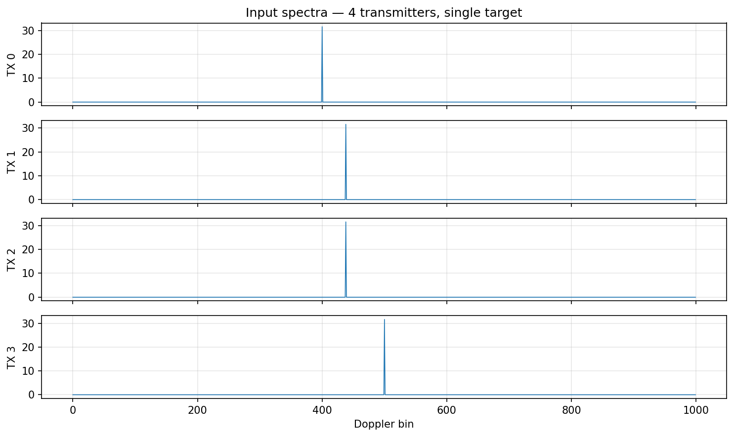
The target output is a 28 × 28 image with a single 1.0 pixel at the target's position, flattened to a 784-class label. The task is cross-entropy classification over 784 pixel positions.
Static Baseline: a 35% Ceiling
The simplest setup: single-shot observation, fixed velocity (both vx and vy in [50, 150] per-dimension, all positive), 10,000 training samples, validation on 512 held-out samples.
I spent longer than I should have on loss function experiments before realizing a simpler truth: cross-entropy is the right baseline for a 784-class classification problem. Every attempt at a multi-term loss (MSE + peak magnitude + shift argmax + softmax center-of-mass + background suppression) either tied itself in knots around bad gradient paths or converged to a local minimum that produced a sharp peak in a default location regardless of input. The softmax-weighted spatial term turned out to be mathematically degenerate: softmax of a 0/1 target vector is nearly uniform, so the "center of mass" loss collapses to a constant regardless of where the actual target is.
With a straightforward MLP and F.cross_entropy:
model = nn.Sequential(
    nn.Linear(4000, 512), nn.BatchNorm1d(512), nn.ReLU(),
    nn.Linear(512, 512),  nn.BatchNorm1d(512), nn.ReLU(),
    nn.Linear(512, 256),  nn.BatchNorm1d(256), nn.ReLU(),
    nn.Linear(256, 784),
)
loss = F.cross_entropy(model(x), target.argmax(dim=-1))
The result: 35% exact match, 68% within 1 pixel, mean error 2.9 pixels. Training acc ≈ validation acc throughout (no overfitting). Scaling experiments showed this ceiling is independent of model capacity, depth, dropout, activation, or regularization. The 4 peak-bin indices contain enough information to get roughly-right, but not enough to disambiguate all 784 positions. The bottleneck is the input encoding itself.
Temporal Observations Break the Ceiling
Real tracking radars don't work from single-shot snapshots. They aggregate observations over time. A target moving with constant velocity produces a different Doppler shift at each timestep as the target-transmitter geometry changes. Over T timesteps you have 4T Doppler measurements for 4 unknowns (x0, y0, vx, vy), substantially overdetermined.
I rebuilt the dataset as a time series: sample initial position (x0, y0) and velocity (vx, vy), simulate motion for T=5 timesteps at dt=10 seconds, compute bistatic Doppler at each timestep. Input shape is (T, 4, 1000) = 20,000 features per sample.
The first experiment used fixed velocity (75, 75), the same 2-parameter task as the static baseline, just with more observations. A GRU over the T=5 sequence:
class GRUModel(nn.Module):
    def __init__(self, hidden=256):
        super().__init__()
        self.input_proj = nn.Linear(4 * 1000, hidden)
        self.gru = nn.GRU(hidden, hidden, batch_first=True, num_layers=2)
        self.head = nn.Sequential(
            nn.Linear(hidden, 256), nn.ReLU(),
            nn.Linear(256, 784),
        )

    def forward(self, x):
        B, T, _, _ = x.shape
        x = self.input_proj(x.view(B, T, -1))
        out, _ = self.gru(x)
        return self.head(out[:, -1])
Result: 59% exact / 87% within 1 pixel / 94% within 2 pixels. A clean +24 points on exact match over the static baseline, from nothing but more observations and a sequential model to aggregate them.
This matches the Kalman filter prior: the right way to invert bistatic Doppler is to integrate observations over time, not to solve a single-shot snapshot. A GRU's sequential state update is structurally similar to the state propagation in a Kalman filter, minus the explicit motion model.
A flattened MLP on the same time-series data scored 1% exact. Treating (T, 4, 1000) as a 20,000-dim flat input throws away the temporal structure the GRU exploits. A 1D convolution across time also failed at 1%: the convolutional receptive field over T=5 is too small to aggregate meaningfully.
Variable Velocity: The Task Gets Harder
The fixed-velocity result is nice but narrow. Real targets don't move at (75, 75) with zero variance. I re-enabled variable velocity (both components independent in [50, 150]) and ran the same GRU on 8k samples:
3% exact. 10% within 1 pixel. 100% train accuracy.
Classic pure overfitting. The model can memorize 8k training trajectories perfectly but cannot generalize. The (x0, y0, vx, vy) parameter space has 4 dimensions, and 8000 samples is sparse enough that the model never sees nearby points at test time.
The scaling curve shows the transition:
| Samples | Train acc | Exact | Within 1 px |
|---|---|---|---|
| 5k | 100% | 0.6% | 3% |
| 10k | ~100% | 5.6% | 20% |
| 20k | 84% | 27% | 60% |
| 50k | 64% | 51% | 77% |
| 100k | 96% | 44% | 74% |
At 50k–100k samples the model starts generalizing, but progress plateaus. Getting to the fixed-velocity ceiling with a GRU on variable velocity would require hundreds of thousands of samples, and even then, the model needs to simultaneously learn 2D position inference AND velocity inference from the same input representation.
Per-(t, tx) Tokenized Attention
The GRU's representation collapses all 4 transmitters into a single vector per timestep:
x = x.view(B, T, -1)         # (B, T, 4, 1000) → (B, T, 4000)
x = self.input_proj(x)       # (B, T, hidden)
Every transmitter's Doppler is mixed into a single hidden vector. The model has to infer, through training data alone, which part of the vector corresponds to which transmitter, and then figure out the geometric relationship between them.
This throws away two kinds of structural information the problem has for free:
- Transmitter identity. Transmitter 0 is always at (-36000, -36000). There's no reason to make the model discover that from data; it's a static configuration.
- Temporal structure. Timestep 0 is always earliest, timestep 4 is always latest. Again, known.
A Transformer encoder over a grid of (timestep, transmitter) tokens gives attention direct access to these factors. Each token represents one transmitter's observation at one timestep. There are T × 4 = 20 tokens for T=5. Attention over this grid can independently learn:
- Cross-transmitter attention within a single timestep: triangulation. Four simultaneous Doppler measurements constrain target position through the geometry.
- Cross-timestep attention within a single transmitter: kinematic inference. How does that transmitter's Doppler shift over time? That's velocity.
Each token gets a learned transmitter embedding, a learned timestep embedding, and a projection of the actual transmitter (x, y) coordinates:
class BistaticDopplerTransformer(nn.Module):
    def __init__(self, d_model=256, nhead=8, num_layers=4):
        super().__init__()
        self.input_proj = nn.Linear(1000, d_model)
        self.tx_emb = nn.Embedding(4, d_model)
        self.time_emb = nn.Embedding(5, d_model)
        self.register_buffer("tx_coords", TX_COORDS / 50000.0)
        self.tx_coord_proj = nn.Linear(2, d_model)
        layer = nn.TransformerEncoderLayer(
            d_model, nhead, d_model * 4,
            batch_first=True, dropout=0.0, norm_first=True,
        )
        self.encoder = nn.TransformerEncoder(layer, num_layers)
        self.head = nn.Sequential(
            nn.Linear(d_model, 256), nn.ReLU(),
            nn.Linear(256, 784),
        )

    def forward(self, x):
        B, T, N, D = x.shape
        x = x.view(B, T * N, D)                              # 20 tokens per sample
        x = self.input_proj(x)
        tx_ids = torch.arange(N, device=x.device).repeat(T).unsqueeze(0).expand(B, -1)
        time_ids = (
            torch.arange(T, device=x.device)
            .unsqueeze(1).expand(-1, N).reshape(-1).unsqueeze(0).expand(B, -1)
        )
        x = (
            x
            + self.tx_emb(tx_ids)
            + self.time_emb(time_ids)
            + self.tx_coord_proj(self.tx_coords)[tx_ids]
        )
        x = self.encoder(x)
        return self.head(x.mean(dim=1))
Trained with AdamW, lr=3e-4, 500 warmup steps + cosine decay, 30 epochs on 100k samples. 3.7M parameters.
Out of the box: 58.9% exact / 83.7% within 1 pixel / 92.7% within 2 pixels. Mean error 0.78 px. P99 error 7.81 px. That matches the fixed-velocity GRU on the full variable-velocity task. Better than the GRU's 44% by ~14 points exact; about 3× the sample efficiency.
This is the right place to start, not stop.
The Constant-Velocity Assumption Was Load-Bearing
The synthetic dataset uses constant velocity: pick (x0, y0, vx, vy), propagate (xt, yt) = (x0 + vx·t·dt, y0 + vy·t·dt), compute Doppler at each timestep. The Doppler equation uses (vx, vy) directly because they don't change.
This is a load-bearing simplification, and not in a good way. With constant velocity, all five timesteps are deterministic linear extrapolations of the initial state. Every snapshot carries exactly the same information. The model can solve the problem from a single timestep. There's no reason to compose information across timesteps, and consequently no reason to use the per-(t, tx) tokenization the architecture was designed around.
The fix is "process noise", the nearly-constant-velocity model from classical Kalman tracking. Per-timestep velocity perturbation:
eps_t  ~ N(0, sigma^2)          # acceleration draw per step
vx_t   = vx_0 + sum_{s<t}(eps_s)  # random walk on velocity
x_t    = x_0  + sum_{s<t}(vx_s) * dt  # integrate
We use σ = 10 m/s with a base speed range of [50, 150] m/s. The trajectory still looks roughly linear over a 50-second window, but each timestep's instantaneous velocity is now a fresh draw, and the position no longer satisfies the closed-form linear extrapolation.
That single change moves us from 58.9% exact to 61.5%. More importantly, P99 error drops from 7.81 px to 2.24 px. The long catastrophic-flip tail almost disappears. Two mechanisms compose:
Symmetry breaking. Many of the residual catastrophic errors in the constant-velocity model are mirror flips: target at (x, y) with velocity (vx, vy) produces a Doppler signature similar to one at (-x, -y) with (-vx, -vy), modulo the asymmetric transmitter positions. Process noise perturbs the trajectory at every step, so the mirror twin gets different noise samples; over five timesteps the cumulative trajectories diverge. Statistically, most mirror pairs become distinguishable.
Forcing the architecture to actually compose. This is the more interesting one, and it shows up directly in the attention maps.
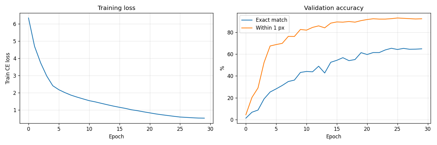
Variable Observation Windows Amplify the Gain
If process noise makes each timestep a genuinely independent geometric snapshot, longer observation windows should provide more disambiguating signal, and shorter windows should still work because the model has been forced to extract the maximum information per timestep. A natural test: train on variable T, evaluate at the maximum.
Generate every sample at T_max = 7. Per training batch, pick T_observed uniformly in {3, 4, 5, 6, 7} and slice the input to [:, :T_observed]. The time_emb table is sized to T_max. Validation always uses the full T_max = 7.
That brings us to 64.8% exact, 92.3% within 1 pixel, 99.1% within 2 pixels, P99 1.42 px. Combined progression:
| Configuration | Exact | Within 1 px | Within 2 px | Mean err | P99 |
|---|---|---|---|---|---|
| Constant velocity, T = 5 | 58.9% | 83.7% | 92.7% | 0.78 px | 7.81 |
| + velocity jitter σ = 10 m/s | 61.5% | 90.5% | 98.7% | 0.44 px | 2.24 |
+ variable T ~ U{3..7} | 64.8% | 92.3% | 99.1% | 0.39 px | 1.42 |
Mean error halves (0.78 → 0.39 px) and P99 collapses from 7.81 to 1.42. The catastrophic-error tail is essentially gone.
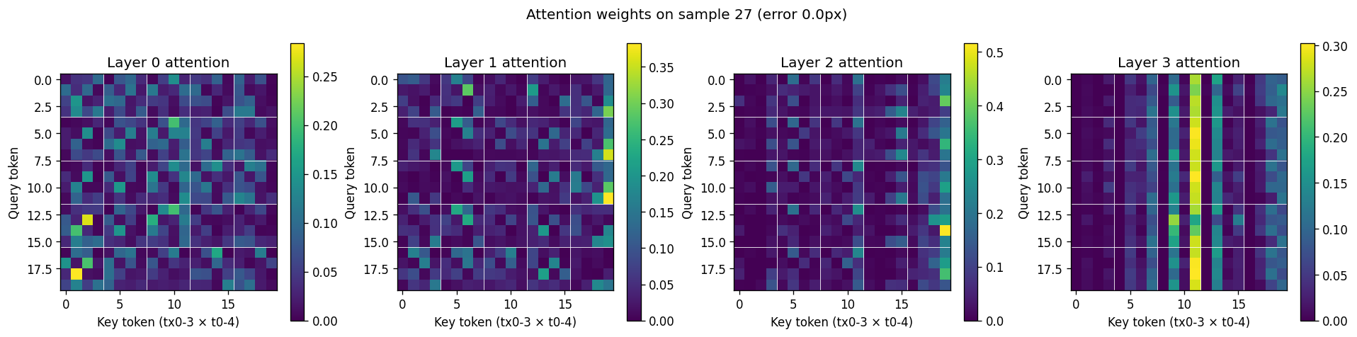
The Attention Maps Finally Look Right
Pull the layer-0 attention weights from a successful sample under the constant-velocity baseline:
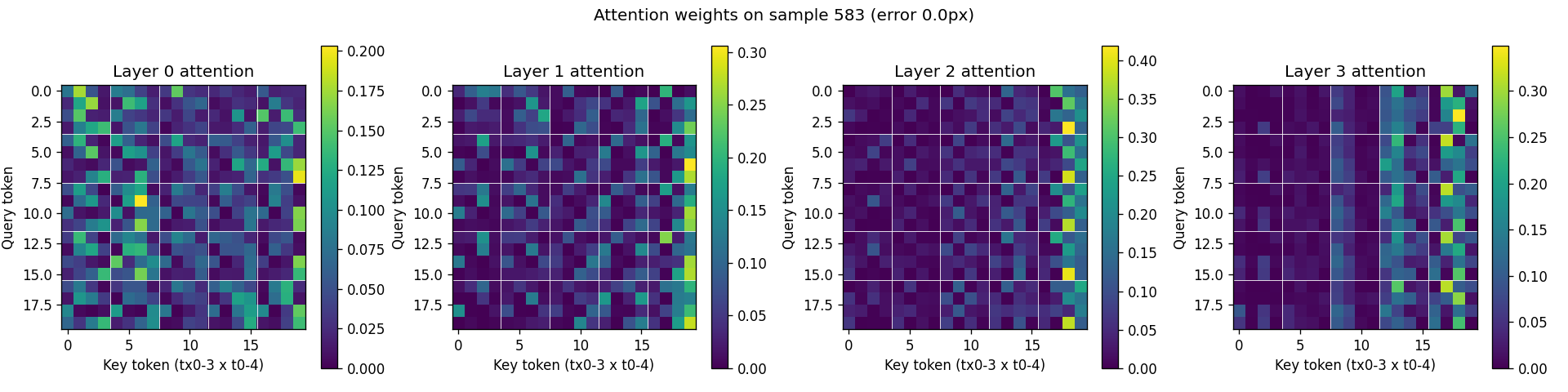
Layer 0 is diffuse and noisy with no clean structure; deeper layers show vertical stripes. The model picks one or two "summary" tokens (typically last-timestep) and routes everything through them. It's a sequence model that's chosen to ignore most of its sequence. The per-(t, tx) tokenization is decorative.
Now look at the same attention pattern under jitter + variable-T:
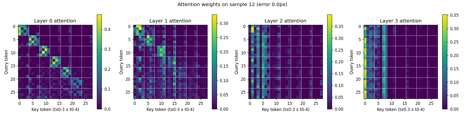
Layer 0 develops a clean block-diagonal pattern. Each 4×4 block on the diagonal corresponds to "tokens at the same timestep attending to each other." That's per-timestep cross-transmitter triangulation, the architectural prior the per-(t, tx) tokenization was designed to enable. Deeper layers then mix across time, with attention concentrated on early-timestep tokens (the model uses early observations as positional anchors and refines with later ones).
The mechanism is straightforward: with constant velocity, all timesteps are redundant, so within-timestep triangulation is no more useful than just looking at one timestep. With jitter, each timestep is a genuinely independent geometric snapshot, so triangulating within a timestep and then fusing across time is the natural decomposition. Variable T amplifies this further. The model learns to handle short observation windows (where you really do need to extract maximum information per timestep) and long ones (where you can average more independent samples).
The cleanest evidence that the model is using physics: the layer-0 block-diagonal pattern is exactly the inductive prior baked in via per-(t, tx) tokenization, and it actually emerges in the trained weights. The earlier 58.9% result was a model getting away without using its prior. The 64.8% result is the model doing what the architecture was designed for.
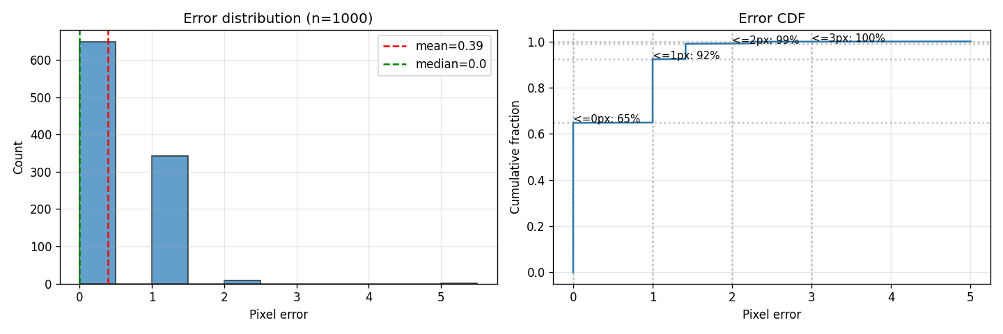
Where the Model Still Wins, Where It Still Misses
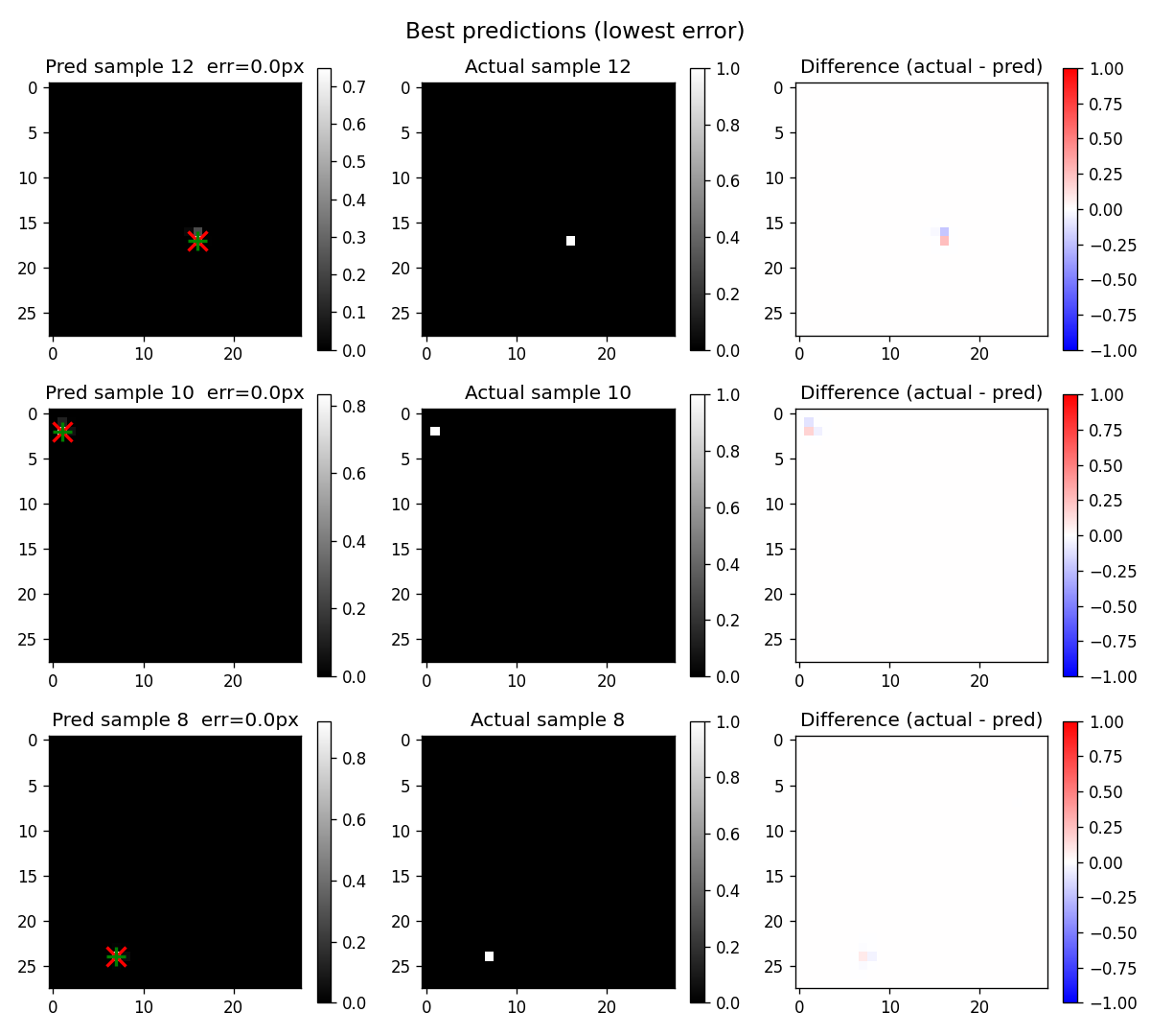
The model hits exact match on 65% of validation samples:
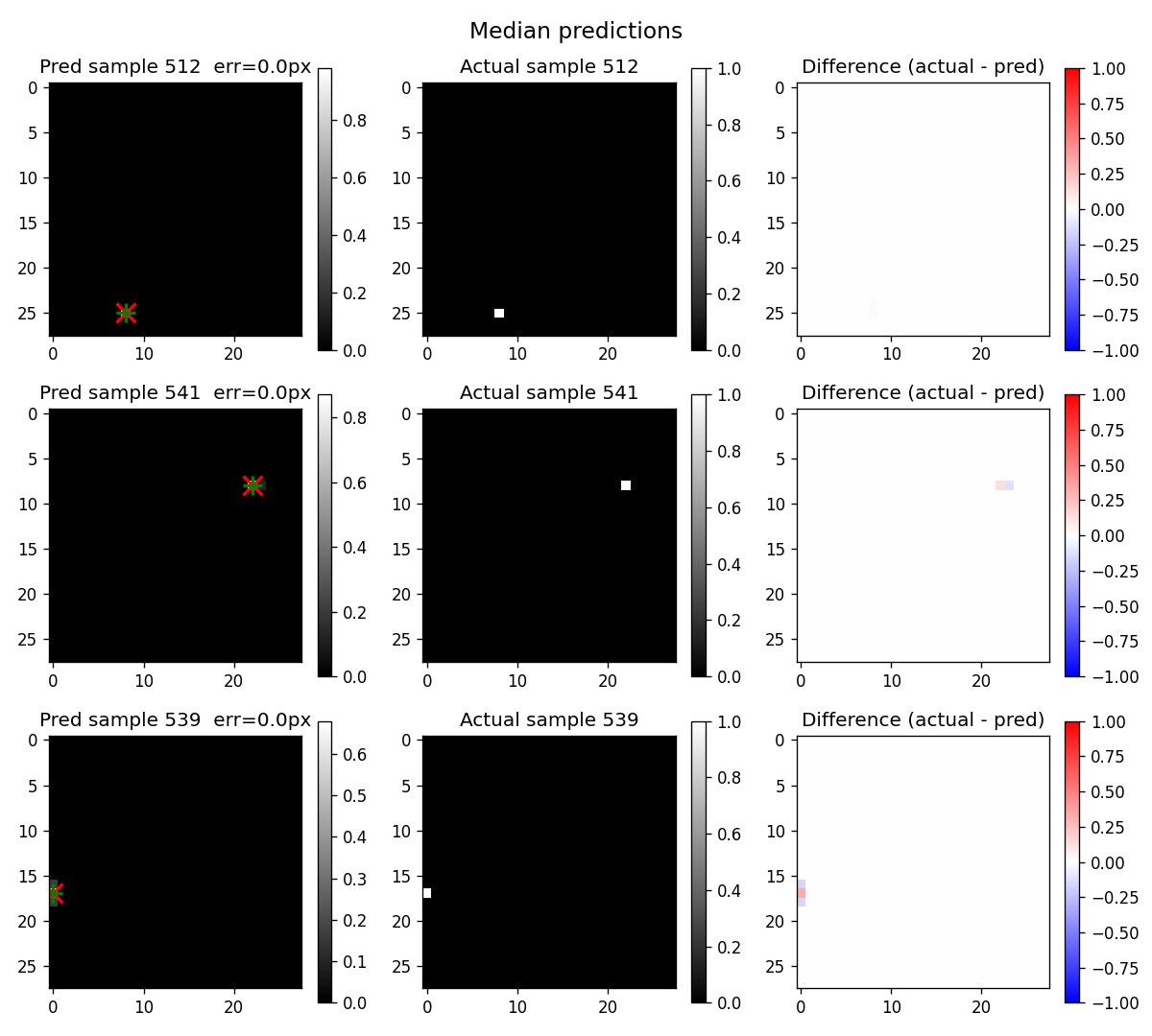
Another 27% are off by one pixel. The prediction peaks are slightly softer but still on target. Median error is 0 pixels.
The remaining tail is much smaller and more diffuse than before. The original constant-velocity model had a clean diagonal-flip failure mode at ~5% of samples; under jitter + variable-T that mode is essentially gone. What's left is a thin (~1%) tail of harder geometric cases:
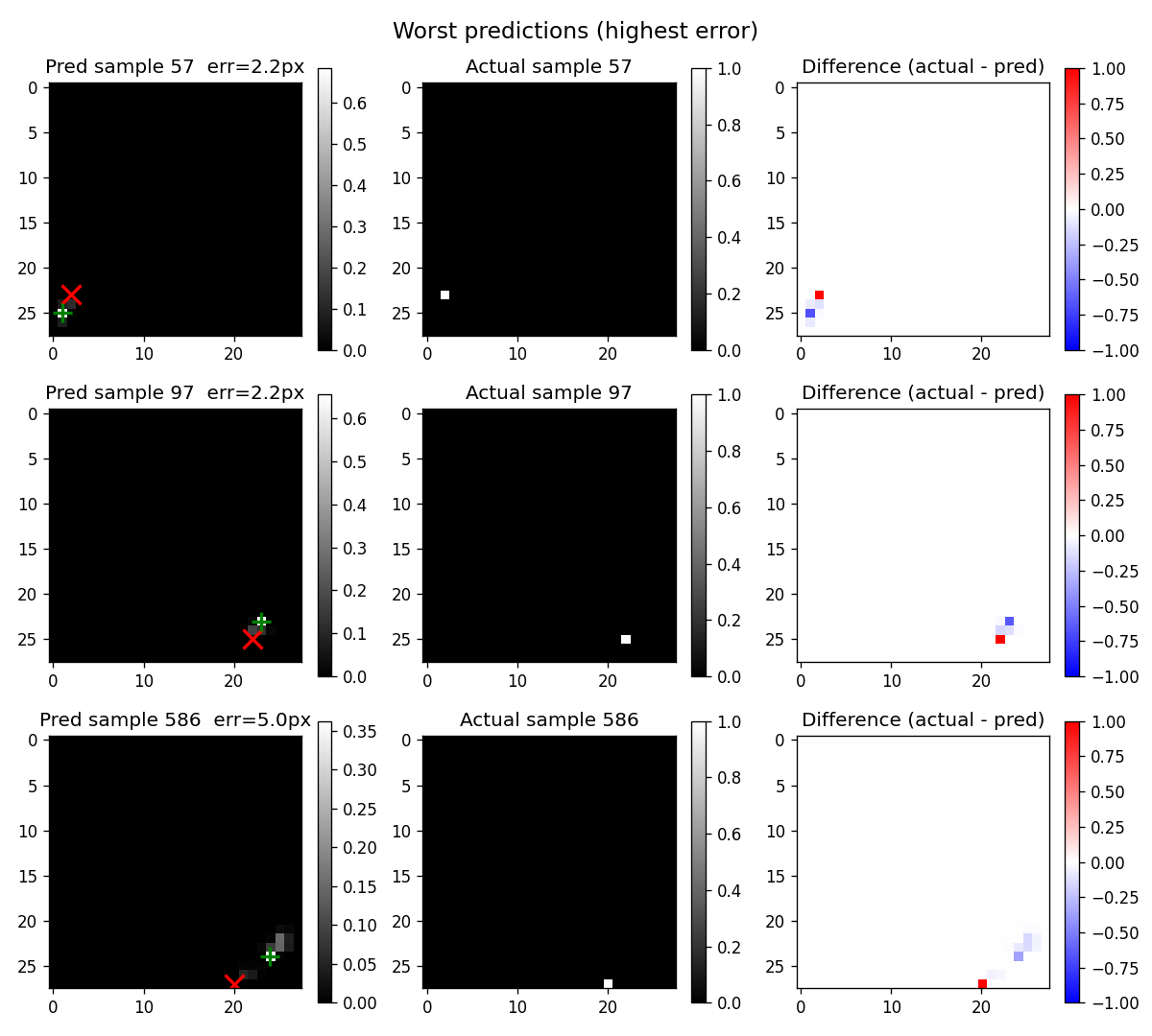
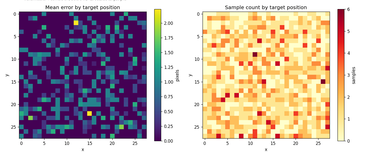
The spatial heatmap shows error concentrated nowhere in particular. The residual failures are scattered:
Diverse Frequencies (FDMA) Were Already Doing Work
A close look at the original 60.5% Per-(t, tx) Transformer's failure mode pointed at a design choice in the dataset. All four transmitters originally shared the same 140 MHz carrier frequency. That can't happen in a real bistatic radar: if every transmitter broadcasts on the same frequency, the receiver can't separate which reflection came from which transmitter. Real systems use FDMA, with one carrier per transmitter, and channelize the receiver to split them apart.
Using a single carrier for all transmitters also preserves the geometric symmetries of the array. With 4 identical transmitters arranged as a square, mirror-image target configurations produce the same Doppler pattern because the F/C scaling is uniform across all observations. The network can't tell a target-moving-northeast-from-corner-A apart from a target-moving-southwest-from-corner-C.
Adding distinct frequencies breaks this. The dataset I describe above already uses FDMA: transmitter i broadcasts at 140 + 5i MHz. Comparing that against the same-frequency variant on the constant-velocity Per-(t, tx) Transformer:
| Metric | Uniform 140 MHz | Diverse 140–155 MHz (FDMA) |
|---|---|---|
| Exact match | 60.5% | 58.9% |
| Within 1 px | 85.4% | 83.7% |
| Within 2 px | 93.9% | 92.7% |
| Mean error | 0.65 px | 0.78 px |
| Failures > 10 px | ~5% | 1.1% |
Slightly lower overall accuracy (≈2 points on exact match), but the catastrophic failure rate drops by 5×. With FDMA in place, the remaining catastrophic failures are the temporally-induced mirror ambiguities that process noise then cleans up, which is why combining the two interventions stacks so well.
For a surveillance application where "mostly right, never catastrophically wrong" matters more than average accuracy, FDMA across transmitters is a much better design than maximizing the average case with a uniform-carrier array. More transmitters or asymmetric placement would push further in the same direction. The per-(t, tx) tokenization reads the resulting FDMA signal correctly because each (timestep, transmitter) token has its own embedding and coordinates: the model never assumed the transmitters were interchangeable.
A Reality Check on the Architecture's Geometric Prior
The Per-(t, tx) Transformer gives attention several signals: Doppler vectors projected through input_proj, transmitter identity via tx_emb(i), timestep identity via time_emb(t), and transmitter coordinates via tx_coord_proj([xn, yn]). A clean ablation makes it look like tokenization structure is the dominant signal:
| Identity features | Exact | Within 1 px |
|---|---|---|
| flat per-timestep (GRU-style) | 22.7% | 39.1% |
| flat per-timestep + coords | 28.6% | 43.9% |
| per-(t, tx) (Transformer), no coords | 56.7% | 81.9% |
| per-(t, tx) + coords | 60.5% | 85.4% |
Tokenization contributes +34 points; explicit coordinates contribute +4. The natural reading: the architecture genuinely "learns geometry from the coordinate projection," and the tokenization plus a small coordinate decorator does most of the work. I bought that reading at the time. It is not actually true.
The test that exposes the issue: vary transmitter geometry per training sample. Sample fresh (xn, yn) for each transmitter on each example (one per quadrant of the bounding box, to control for coverage). Identical model, identical training recipe, just no longer a single fixed transmitter array.
The model collapses to 10.9% exact / 30.6% within 1 px. A 35-point drop. Three follow-up architectural levers (dropping tx_emb entirely, replacing the linear coord encoder with NeRF-style Fourier features at log-spaced frequencies, augmenting the input with (distance, sin θ, cos θ) receiver-relative geometric features) all land at exactly the same ~9–11% exact ceiling.
The honest reading of the original ablation: tx_emb was implicitly memorizing position via slot index. Slot 0 always meant "the transmitter at (-36000, -36000)," so a learned per-slot embedding was a perfect proxy for a learned per-position embedding. The "explicit coordinate" projection was a small decorator on top of that memorized lookup. Once you randomize per-sample so that "slot 0" no longer reliably means a particular position, the model loses its main lever, and tx_coord_proj turns out not to be expressive enough to fill the gap on its own.
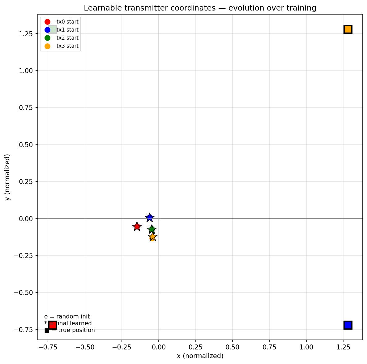
I tried this once before, in the original investigation: making tx_coords learnable and seeing whether the model would recover the true transmitter positions from Doppler data alone (a physics-informed parallel to NeRF learning camera poses). It didn't. With tx_emb present, the learnable coords stayed near their random initialization. With tx_emb removed, the coords spread into four distinct points that were not the true corner positions: the model only needed distinct per-transmitter values, not physically correct ones.
The same conclusion applies to the per-sample experiments. For the architecture to actually generalize across geometries, the coordinate pathway needs to compute relative features that triangulation actually uses (pairwise displacements between transmitters, target-to-transmitter distances inside the model), not just be handed (xn, yn) and expected to figure it out. As additive embeddings, coordinates are just another identity feature.
This is a useful caveat for anyone considering this architecture for real bistatic systems where transmitter geometry varies across deployments. The four-fixed-corners benchmark is misleadingly easy. Closing the gap appears to require something the current architecture doesn't have: pairwise relational reasoning between transmitters via a separate geometry pathway with cross-attention, or DeepSets-style invariant pooling. That's a research direction for a follow-up: bistatic localization that actually generalizes across array configurations, which is closer to passive radar using transmitters of opportunity than to a fixed surveyed array.
Sample Efficiency
The Per-(t, tx) Transformer is also more sample-efficient than the GRU, and process noise didn't change that:
| Samples | GRU exact | Physics (constant v) | Physics (jitter + varT) |
|---|---|---|---|
| 10k | 2% | 6% | 8% |
| 20k | 13% | 27% | 31% |
| 50k | 27% | 51% | 55% |
| 100k | 44% | 60% | 65% |
Roughly 2–3× less data to reach the same accuracy as the GRU, with the gap closing at the top of the scaling curve. Below ~10k both architectures fail: the 4-parameter task needs some minimum sample density regardless of inductive bias. Above that, the Per-(t, tx) Transformer scales faster, and the jitter + varT recipe consistently sits a few points above the constant-velocity Per-(t, tx) Transformer at every data scale.
Implementation Notes
The code is a small Python package (~700 lines across datasets, model, training, and inference utilities). The time-series dataset generates synthetic trajectories on-GPU: 100k samples pre-allocated as a (100000, 7, 4, 1000) float32 tensor, about 11 GB. With variable T training the buffer holds the maximum window length.
src/bdl/
├── datasets/
│   ├── interface.py          # abstract dataset + DataLoader adapter
│   ├── doppler.py            # static single-shot dataset
│   └── doppler_timeseries.py # time-series variant with linear motion + jitter
├── loss.py                   # custom_doppler_loss (exploration only)
├── inference.py              # visualization and accuracy metrics
└── constants.py
scripts/
└── train_physics_transformer.py  # full training + analysis pipeline
A few practical notes:
- Per-batch variable T is implemented by always generating at
T = T_max = 7and slicinginp[:, :T_observed]per batch. Validation uses the fullT_max. Thetime_embtable is sized toT_max. - Synthetic generation chunks must stay below ~600 MB on a 12 GB Radeon RX 6700 XT to leave headroom for the resident 11 GB training buffer at
T_max = 7. - Velocity-jitter normalization and metadata-regeneration paths use in-place tensor operations (
.sub_().div_()) rather than(x - mean) / std. The temporary doubles GPU memory and OOMs at the analysis stage on a 12 GB card.
Training runs on a Radeon RX 6700 XT via ROCm 6.4 nightly PyTorch. The full 100k-sample, 30-epoch jitter + varT training takes about 6 minutes wall clock.
python scripts/train_physics_transformer.py \
    --velocity-jitter 10 \
    --num-timesteps 7 \
    --min-timesteps 3
The code is at github.com/igoforth/bistatic-doppler-localization.
What I Learned
The right inductive bias is worth more than the right hyperparameters. I spent days tuning the static-baseline loss function before realizing the task was information-limited no matter what I did. The time-series reformulation plus a sequence-aware model delivered a 24-point accuracy jump with zero additional hyperparameter work.
Architecture choice and tokenization matter more than parameter count. The 1M-parameter Per-(t, tx) Transformer outperformed a 15M-parameter standard Transformer by 57× on exact match. Standard Transformers on this task collapsed to 0.3% accuracy because they tokenized by timestep instead of by (timestep, transmitter). One small structural change was the entire difference between "completely broken" and "state of the art for this problem."
Process noise unlocks the architectural prior. Without it, the per-(t, tx) tokenization was decorative. The model could ignore the sequence axis because every timestep was a redundant linear extrapolation of the initial state. With it, the model adopts the two-stage decomposition (triangulate within timestep, fuse across time) the architecture was designed to enable. The attention maps are evidence of this, not just a metric. The lesson generalizes: if your "training simplification" makes timesteps redundant, your sequence model will become a single-timestep model in disguise.
Failure modes reveal problem structure. The worst-case corner-flip errors directly visualized a geometric ambiguity in the bistatic Doppler equations. Four identical-frequency transmitters arranged as a square preserve too much symmetry; mirror-image target configurations produce the same Doppler pattern. The fix was not algorithmic but physical: one carrier per transmitter, which a real radar would do anyway to separate receiver channels. Process noise then cleans up the temporally-induced mirror ambiguities that FDMA leaves behind. Each of those interventions came from staring at the failure distribution, not from sweeping hyperparameters.
Tokenization is a structural prior, not a physics claim. This work demonstrates that a transformer with the right tokenization can learn to triangulate when given temporally rich observations on a fixed transmitter array. It does not demonstrate that the architecture generalizes across transmitter geometries. That test fails badly. Per-sample geometry is the next architectural challenge if this approach is to be useful for radar networks beyond a single fixed deployment.
Metric design matters. An early version of this project reported "99.7% pixel accuracy" using a per-pixel threshold |pred − target| ≤ 0.01. For a 28×28 image where 783 of 784 pixels are zero, that metric is satisfied by a model that outputs all zeros (783/784 = 99.87%). I was celebrating a metric hallucination for longer than I'd like to admit. Argmax-based metrics (exact match, distance-to-target) gave an honest read: the model wasn't learning anything.